Example Problem in Autolev and Ch
Problem
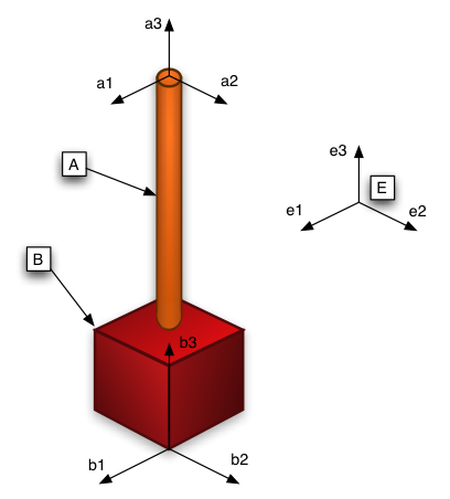
The system analysed here is a compound pendulum. It consists of a slender rod, A, that swings swings in the reference frame, E, about the horizontal unit vector e1. The a1 unit vector of the reference frame fixed in A points in the same direction as the e1 unit vector. Attached to the bottom of A is a body B that rotates about the a3 and b3 unit vectors, with the b unit vectors fixed in B. A only has a moment of inertia about the a1 axis. B has different moments of inertia about each of its 3 axes. Friction is neglected. This problem is designed to show how differences in initial conditions can effect the ensuing motion of the system. For all of the code on this page, there is a link where you can view/download the code as a simple text file.
Autolev
The Autolev code for this problem is very straight forward. The only force is gravity. It is the different moments of inertia for B that make this problem interesting.
% pendulum.al
%
% Variable Definition
%
newtonian e
bodies a, b
constants la, lb, g
variables q{2}', u{2}'
%
% Mass Properties
%
mass a = ma, b = mb
inertia a, a1
inertia b, b1, b2, b3
%
% Generalized Speeds
%
q1' = u1
q2' = u2
%
% Kinematics
%
simprot(e, a, 1, q1)
simprot(a, b, 3, q2)
w_a_e> = q1'*a1>
w_b_e> = w_a_e> + q2'*b3>
v_ao_e> = la*q1'*a2>
v_bo_e> = lb*q1'*a2>
alf_a_e> = dt(w_a_e>, e)
alf_b_e> = dt(w_b_e>, e)
a_ao_e> = dt(v_ao_e>, e)
a_bo_e> = dt(v_bo_e>, e)
%
% Forces
%
gravity(-g*e3>
f = fr()
fstar = frstar()
zero = fr() + frstar()
kane()
solve(zero, [u1', u2'])
output t, q2
output t, q1
units q{1:2} = deg
units u{1:2} = deg/s
units [ma; mb] = kg
units [la; lb] = m
units g = m/s^2
units [a1; b1; b2; b3] = kg*m^2
input ma = 0.01, mb = 0.1
input g = 9.81
input la = 0.075, lb = 0.2
input a1 = 0.000005
input b1 = 0.00025, b2 = 0.00005, b3 = 0.0002
code dynamics() pendulum.c, subs
Program
The program that Autolev creates to simulate this system is close to 400 lines
so I won't show it here. Instead, I've included links to the program files.
The first one is the original C program created in Autolev with by running the
.al file above. The second program has the all the modifications that were
discussed on the main page. There are comments on either side of the added
or modified portions. The last file is just a list of the lines that have been
added or changes so you know where to look.
C code Altered C code Differences
Input
This is the input file showing one set of initial conditions used for this problem. The starting angles for the 4 different cases are as follows:
- A = 45° & B = 0.5°
- A = 45° & B = 1.0°
- A = 90° & B = 0.5°
- A = 90° & B = 1.0°
File: pendulum.in
-----------------------------------------------------------------------------
Case 4: q1(0) = 90.0 and q2(0) = 1.0
----------------------------------------------------------+------------------
Description          Quantity             Units           | Value
----------------------------------------------------------|------------------
Constant:            A1                   KG*M^2          |  0.000005
Constant:            B1                   KG*M^2          |  0.00025
Constant:            B2                   KG*M^2          |  0.00005
Constant:            B3                   KG*M^2          |  0.0002
Constant:            G                    M/S^2           |  9.81
Constant:            LA                   M               |  0.075
Constant:            LB                   M               |  0.2
Constant:            MA                   KG              |  0.01
Constant:            MB                   KG              |  0.1

Initial Value:       Q1                   DEG             |  90.0
Initial Value:       Q2                   DEG             |  1.0
Initial Value:       U1                   DEG/S           |  0.0
Initial Value:       U2                   DEG/S           |  0.0

Initial Time:        TINITIAL             UNITS           |  0.0
Final Time:          TFINAL               UNITS           |  10.0
Integration Step:    INTEGSTP             UNITS           |  0.1
Print-Integer:       PRINTINT             Positive Integer|  1
Absolute Error:      ABSERR                               |  1.0E-08
Relative Error:      RELERR                               |  1.0E-07
----------------------------------------------------------+------------------

DANGER: Do not insert TABS while editing this file.

Note:

  INTEGSTP*PRINTINT is the time-interval for writing of output.

  ABSERR should be set equal to 10^(-8)*Xsmall, where Xsmall is the estimated
         smallest maximum absolute value of the variables being integrated.

  RELERR should be set equal to 10^(-d), where d is the desired number of
         significant digits of numerical integration results.
Output
The data files output by the program will be the same as before it was modified, with one exception. The heading portion will be modified as shown below. Lines starting with # are seen as comments by Ch. This makes it easy to compare the output from different cases.
# FILE: pendulum.1
#
# *** Case 4: q1(0) = 90.0 and q2(0) = 1.0
#
#
#        T             Q2
#     (UNITS)         (DEG)
#
  0.000000E+00   1.000000E+00
  1.000000E-01   9.815411E-01
Plots
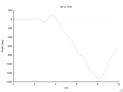
After modification, the program plots the output directly. As can be see above, it will plot to the screen and to a file. This gives the benefit of immediate feedback and saving the plots without any additional steps. You may choose to use a different format for the file output if you don't have a program that can handle an .eps.
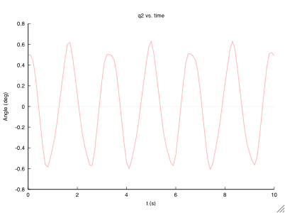
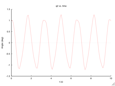
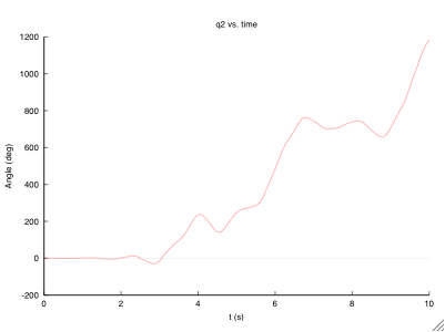
External Plots
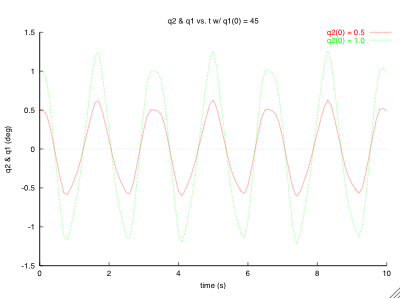
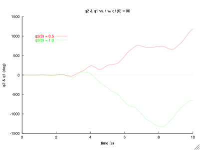
After seeing the results separately, you might want to compare the different cases.
By modifying the data files, you can run the program below to plot the results of many
different files together. The only difference with plot external files is the
.dataFile() function.
/* pendulum_plot.ch */
/* Plotting the output of pendulum.c */
/* Initial values: q1(0) = 90 & q2(0) = 1, 0.5 */

#include <stdio.h>
#include <chplot.h>

int main()
{
   class CPlot plot;
   char *title = "q2 & q1 vs. t w/ q1(0) = 90";
   char *xlabel = "time (s)";
   char *ylabel = "q2 & q1 (deg)";

   plot.dataFile("pendulum_3.1");
   plot.dataFile("pendulum_4.1");
   plot.legend("q2(0) = 0.5", 0);
   plot.legend("q2(0) = 1.0", 1);
   plot.legendLocation(2,1000);
   plot.title(title);
   plot.label(PLOT_AXIS_X, xlabel);
   plot.label(PLOT_AXIS_Y, ylabel);
   plot.plotting();
   plot.outputType(PLOT_OUTPUTTYPE_FILE, "postscript eps color", "plot_34.eps");
   plot.plotting();
   return 0;
}
Here I've shown comparison plots for cases 1 & 2, and cases 3 & 4. They were both created with the above program by making a few minor changes.
Back to Main Page
Autolev™ is the property of OnLine Dynamics, Inc.


